Plotting
This notebook demonstrates all gcmprocpy plotting functions, including projections, wind vector overlays, coastlines, and height-mode plotting.
Note: This notebook requires TIE-GCM or WACCM-X model output files.
[1]:
import warnings
warnings.filterwarnings('ignore')

%matplotlib inline
import numpy as np
import matplotlib.pyplot as plt
import gcmprocpy as gy

directory = '/glade/work/nikhilr/tiegcm3.0/benchmarks/2.5/seasons/decsol_smin/hist'
datasets = gy.load_datasets(directory, dataset_filter='sech')
times = gy.time_list(datasets)
t_val = times[0]
print(f'Using time: {t_val}')
Using time: 2002-12-21T01:00:00.000000000
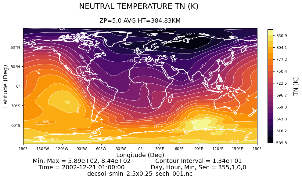
Latitude vs Longitude Contour Plot
[2]:
fig = gy.plt_lat_lon(datasets, 'TN', time=t_val, level=5.0)
plt.show()

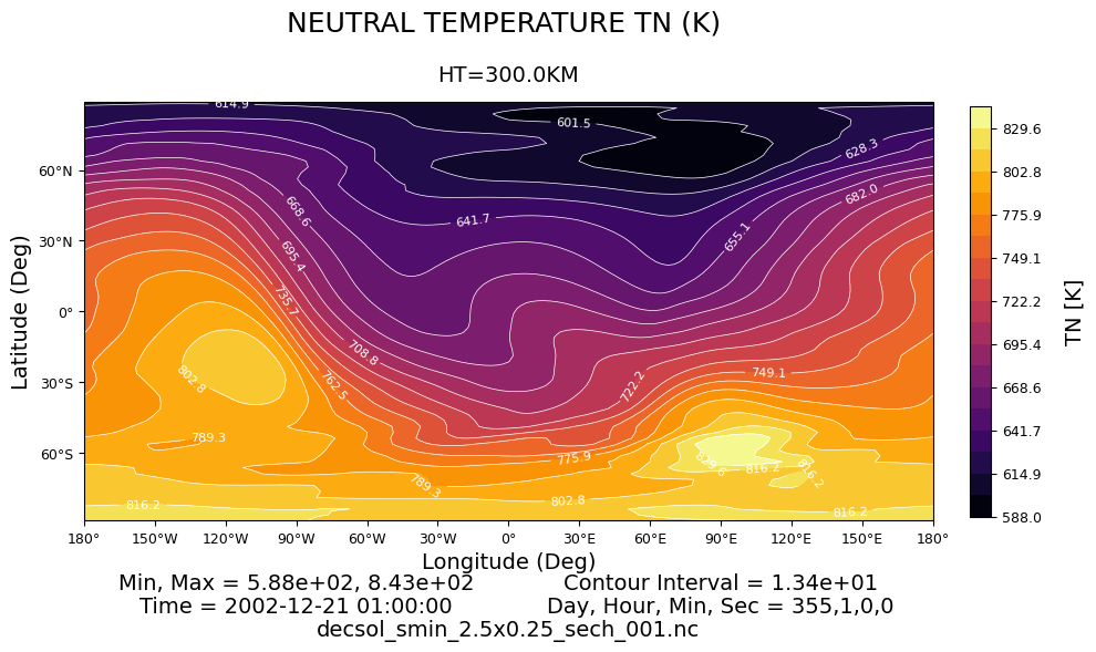
Using Height (level_type='height')
[3]:
fig = gy.plt_lat_lon(datasets, 'TN', time=t_val, level=300.0, level_type='height')
plt.show()
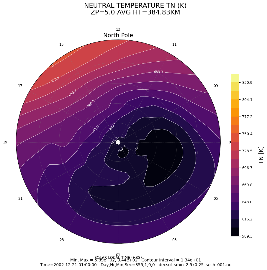
Polar Projections
The projection parameter supports 'north_polar', 'south_polar', and 'polar' (both hemispheres).
[4]:
fig = gy.plt_lat_lon(datasets, 'TN', time=t_val, level=5.0, projection='north_polar')
plt.show()
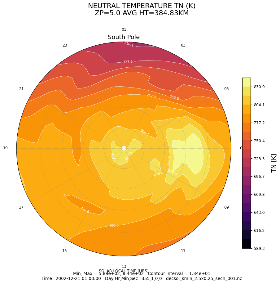
[5]:
fig = gy.plt_lat_lon(datasets, 'TN', time=t_val, level=5.0, projection='south_polar')
plt.show()
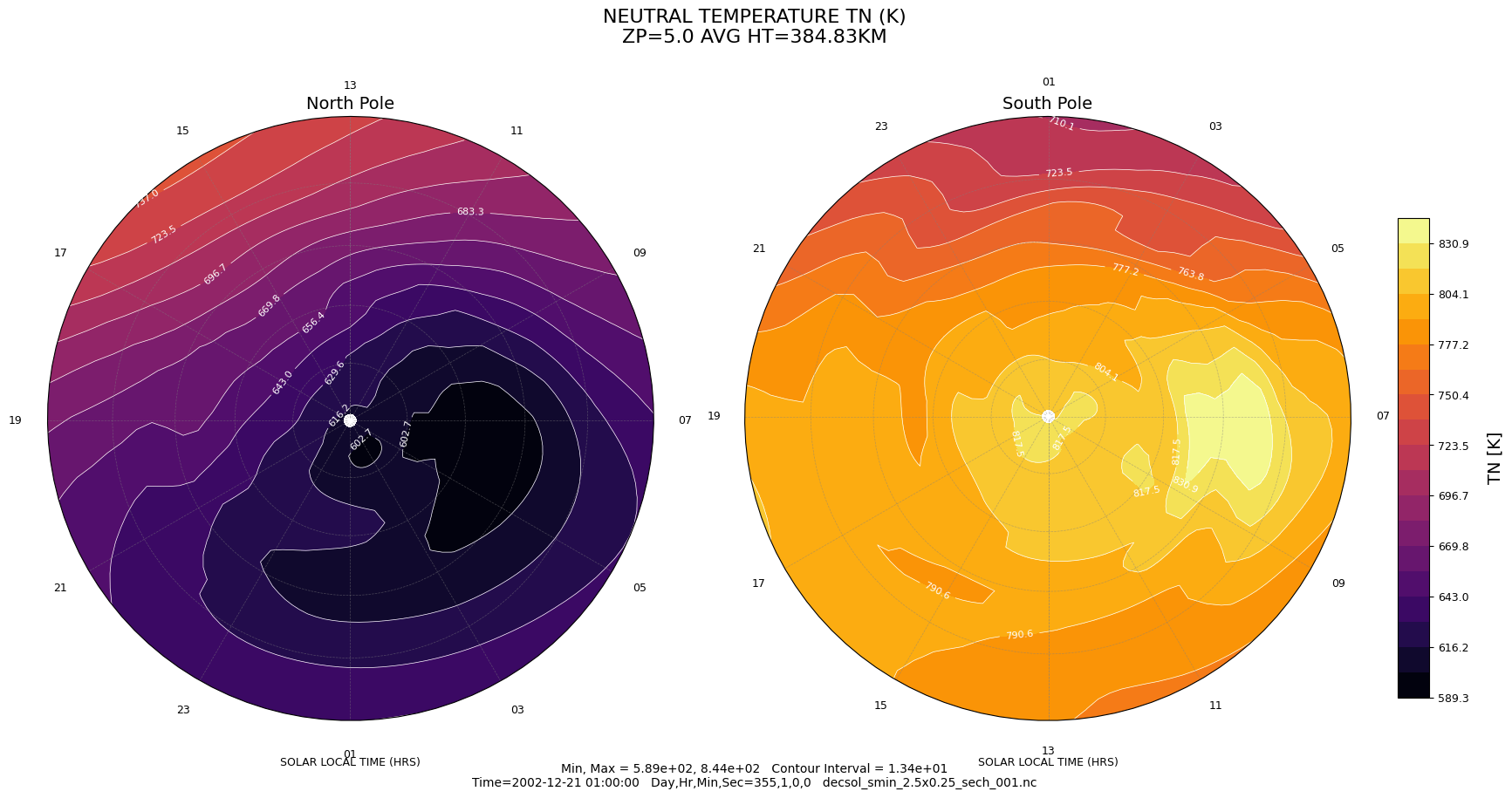
[6]:
fig = gy.plt_lat_lon(datasets, 'TN', time=t_val, level=5.0, projection='polar')
plt.show()
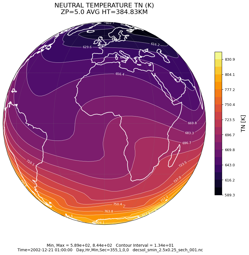
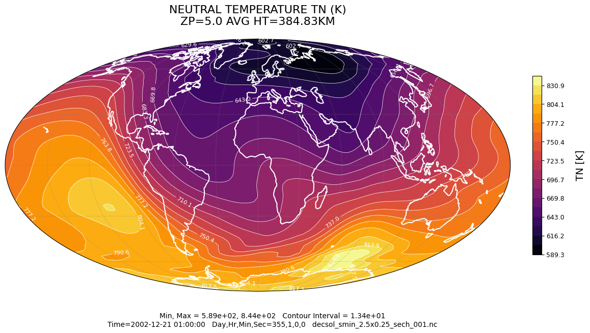
Orthographic and Mollweide Projections
[7]:
fig = gy.plt_lat_lon(datasets, 'TN', time=t_val, level=5.0, projection='orthographic', coastlines=True)
plt.show()
[8]:
fig = gy.plt_lat_lon(datasets, 'TN', time=t_val, level=5.0, projection='mollweide', coastlines=True)
plt.show()
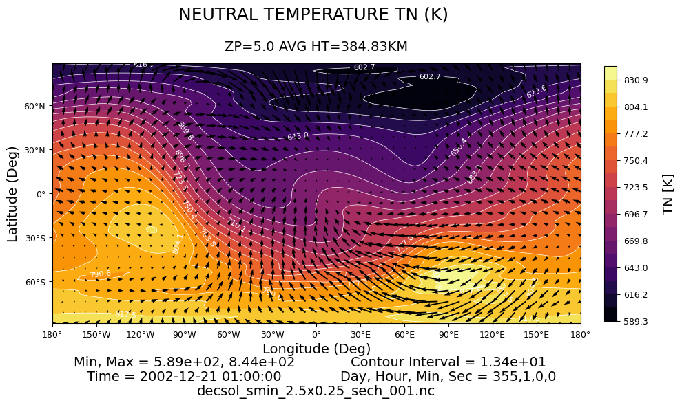
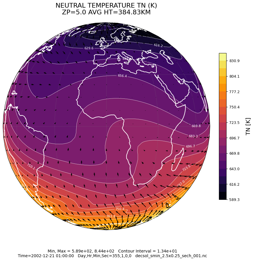
Wind Vector Overlays
Set wind=True to overlay wind vectors. Wind variable names are automatically selected based on model type.
[9]:
fig = gy.plt_lat_lon(datasets, 'TN', time=t_val, level=5.0, wind=True, wind_density=3)
plt.show()
[10]:
fig = gy.plt_lat_lon(datasets, 'TN', time=t_val, level=5.0,
                     projection='orthographic', central_latitude=0,
                     wind=True, wind_density=3, coastlines=True)
plt.show()
Coastlines
[11]:
fig = gy.plt_lat_lon(datasets, 'TN', time=t_val, level=5.0, coastlines=True)
plt.show()
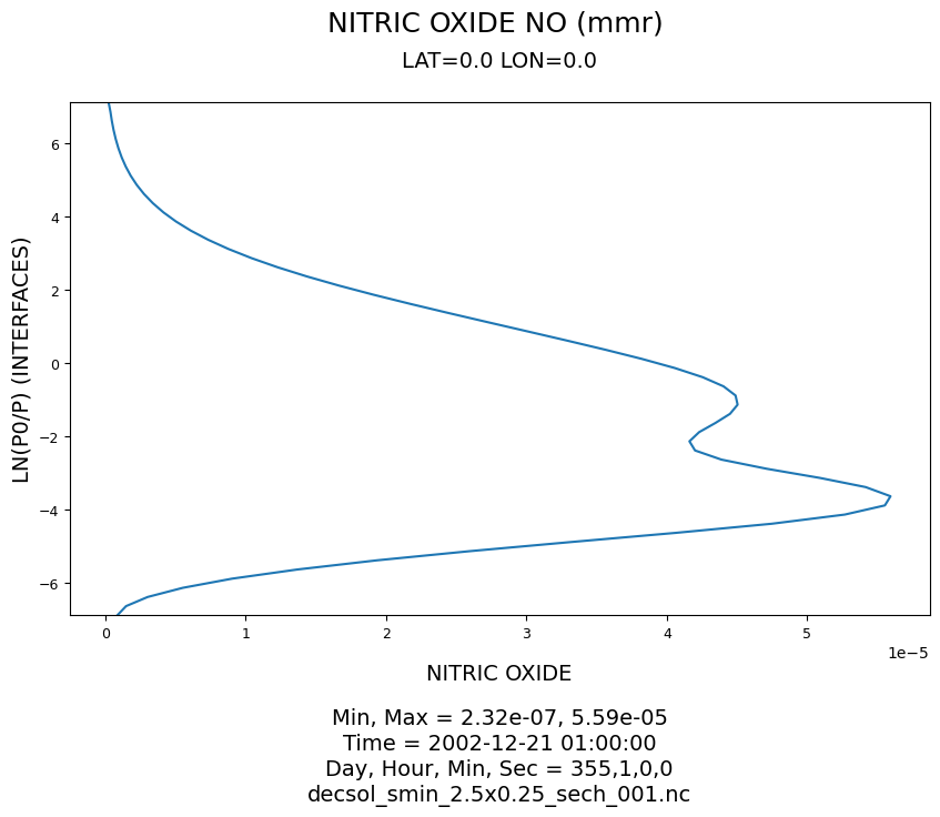
Pressure Level / Height vs Variable Line Plot
[12]:
fig = gy.plt_lev_var(datasets, 'NO', latitude=0.0, time=t_val, longitude=0.0)
plt.show()
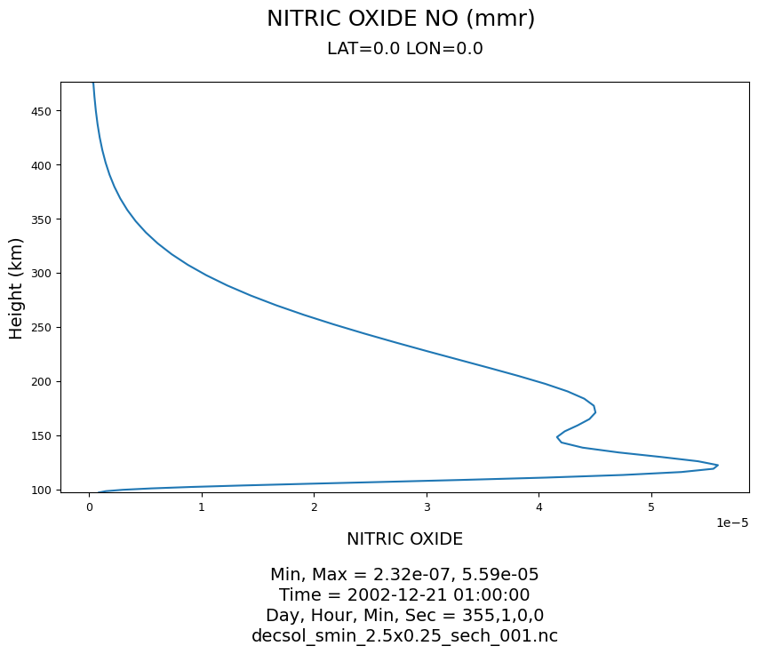
Using y_axis='height' to display the vertical axis in km:
[13]:
fig = gy.plt_lev_var(datasets, 'NO', latitude=0.0, time=t_val, longitude=0.0, y_axis='height')
plt.show()
Variable vs Latitude Line Plot
1D meridional cut at a fixed longitude and pressure level. Pass longitude='mean' (or omit it) to compute a zonal mean.
[14]:
fig = gy.plt_var_lat(datasets, 'TN', level=5.0, time=t_val, longitude=0.0)
plt.show()
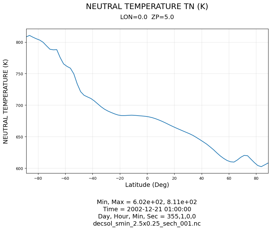
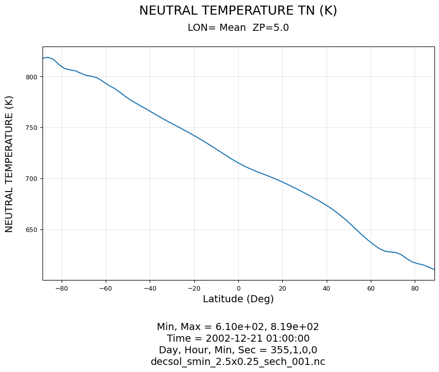
Zonal mean (averaged over all longitudes):
[15]:
fig = gy.plt_var_lat(datasets, 'TN', level=5.0, time=t_val)
plt.show()
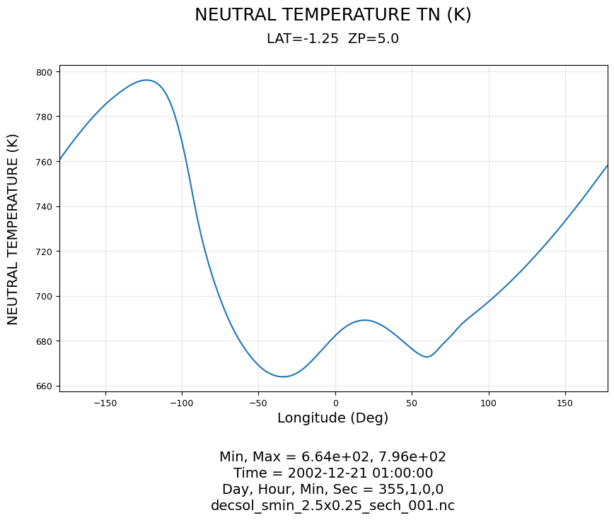
Variable vs Longitude Line Plot
1D zonal cut at a fixed latitude and pressure level. Pass latitude='mean' (or omit it) to compute a meridional mean.
[16]:
fig = gy.plt_var_lon(datasets, 'TN', level=5.0, time=t_val, latitude=0.0)
plt.show()
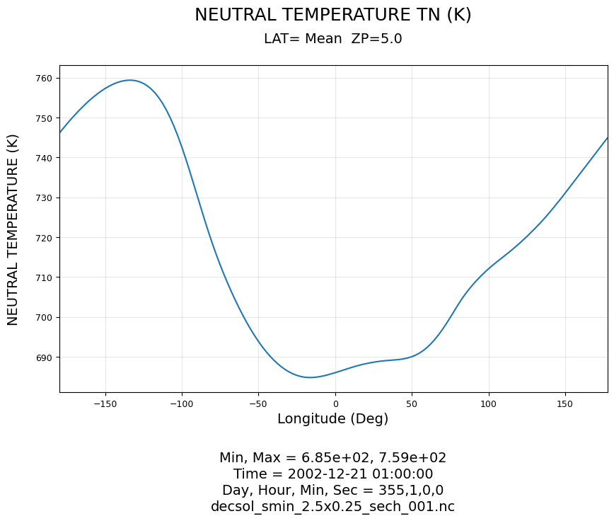
Meridional mean (averaged over all latitudes):
[17]:
fig = gy.plt_var_lon(datasets, 'TN', level=5.0, time=t_val)
plt.show()
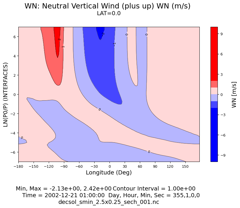
Pressure Level / Height vs Longitude Contour Plot
[18]:
fig = gy.plt_lev_lon(datasets, 'WN', symmetric_interval=True,    latitude=0.0, time=t_val)
plt.show()
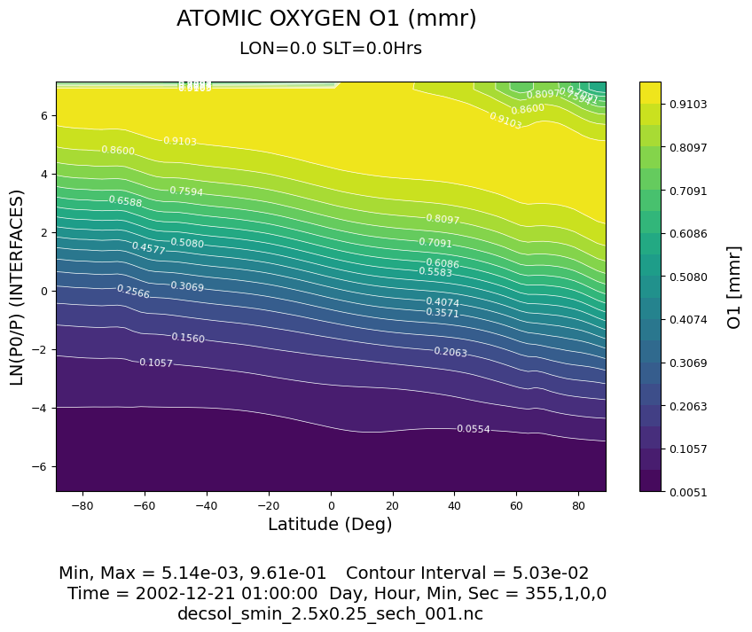
Pressure Level / Height vs Latitude Contour Plot
[19]:
fig = gy.plt_lev_lat(datasets, 'O1', time=t_val, longitude=0.0)
plt.show()
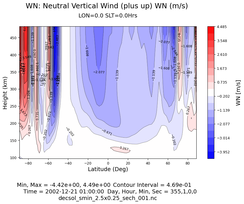
Using y_axis='height':
[20]:
fig = gy.plt_lev_lat(datasets, 'WN', time=t_val, longitude=0.0, y_axis='height')
plt.show()
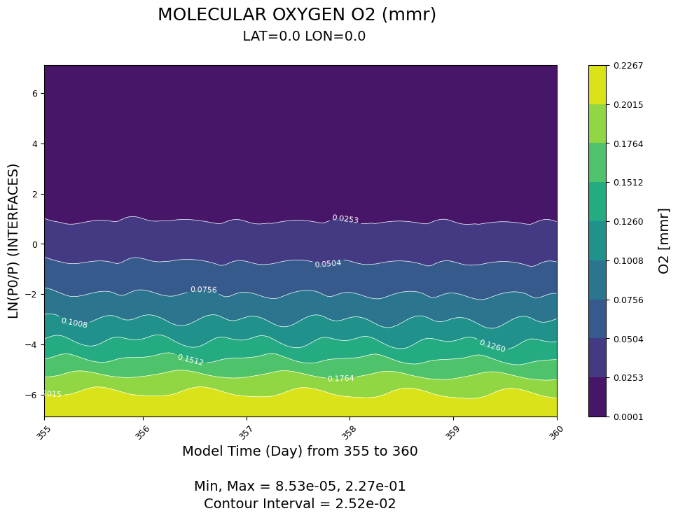
Pressure Level / Height vs Time Contour Plot
[21]:
fig = gy.plt_lev_time(datasets, 'O2', latitude=0.0, longitude=0.0)
plt.show()
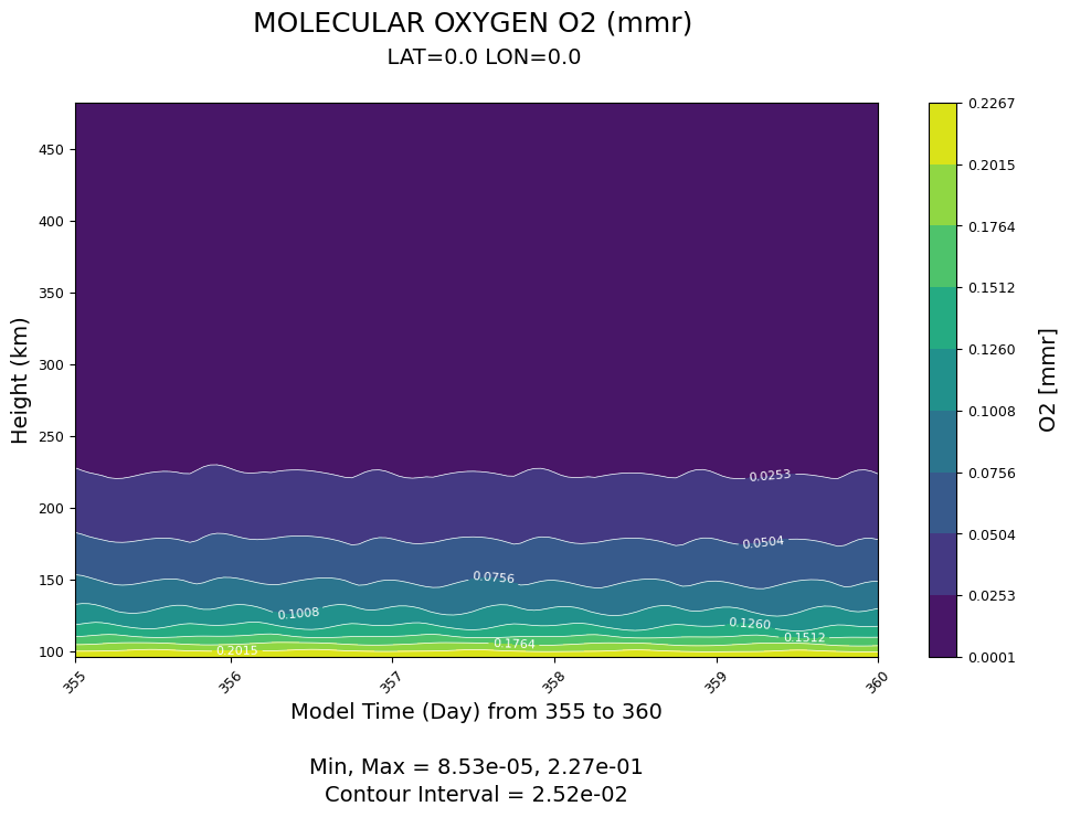
Using y_axis='height':
[22]:
fig = gy.plt_lev_time(datasets, 'O2', latitude=0.0, longitude=0.0, y_axis='height')
plt.show()
Latitude vs Time Contour Plot
[23]:
fig = gy.plt_lat_time(datasets, 'TN', level=5.0, longitude=0.0)
plt.show()

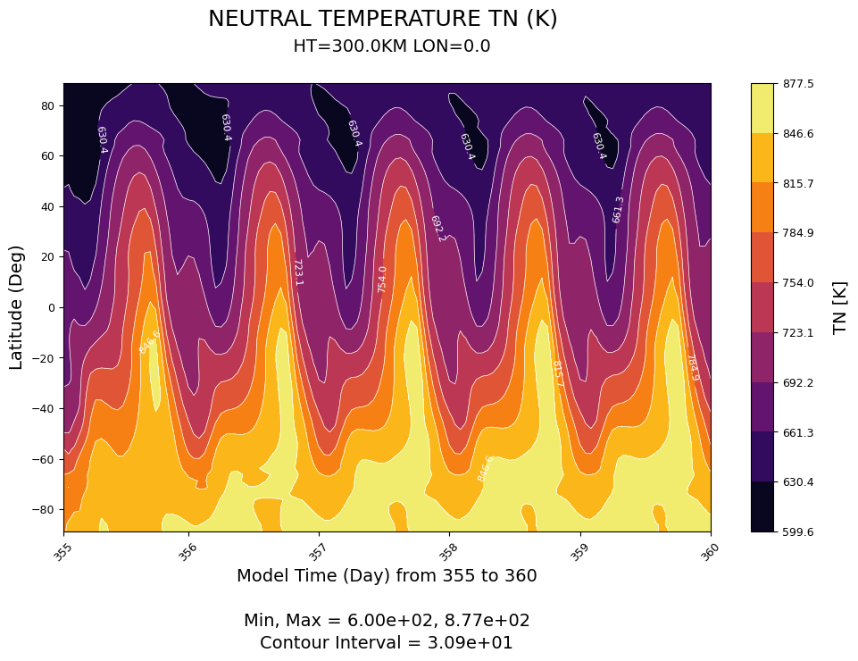
Using level_type='height':
[24]:
fig = gy.plt_lat_time(datasets, 'TN', level=300.0, longitude=0.0, level_type='height')
plt.show()
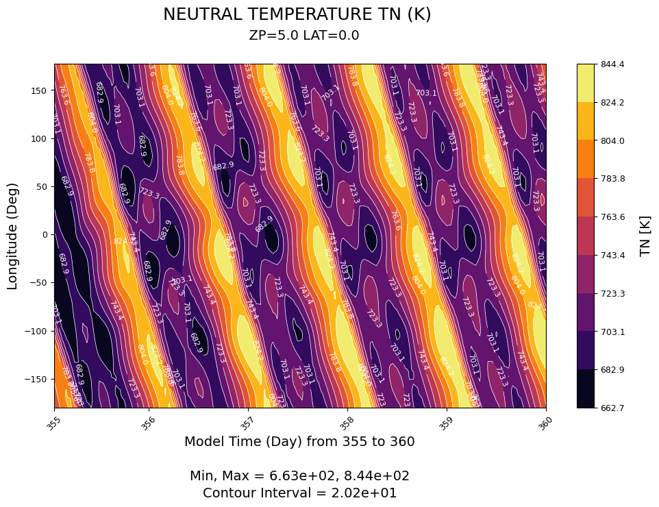
Longitude vs Time Contour Plot
[25]:
fig = gy.plt_lon_time(datasets, 'TN', latitude=0.0, level=5.0)
plt.show()
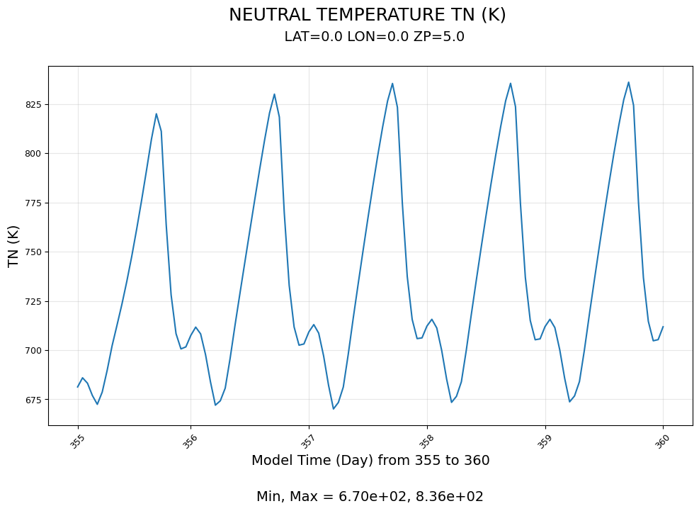
Variable vs Time Line Plot
[26]:
fig = gy.plt_var_time(datasets, 'TN', latitude=0.0, longitude=0.0, level=5.0)
plt.show()
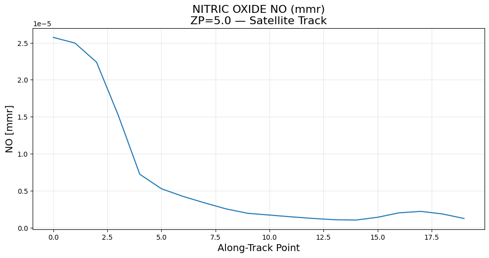
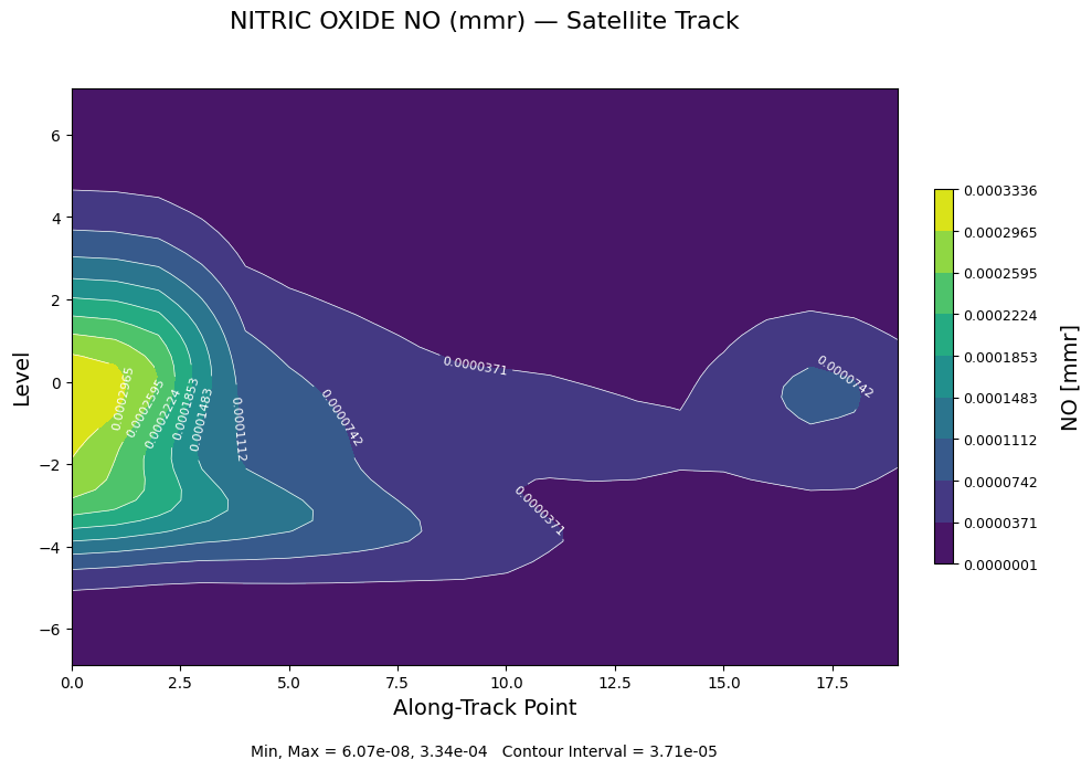
Satellite Track Interpolation Plot
Interpolate model data along a satellite trajectory. With a level specified: 1D line plot. Without: 2D contour plot.
[27]:
# Simulate a LEO ascending pass
sat_time = np.array([times[0] + np.timedelta64(i * 6, 'm') for i in range(20)])
sat_lat = np.linspace(-60, 60, 20)
sat_lon = np.linspace(-120, 120, 20)

# Line plot at a fixed level
fig = gy.plt_sat_track(datasets, 'NO', sat_time, sat_lat, sat_lon, level=5.0)
plt.show()
[28]:
# Contour plot across all levels
fig = gy.plt_sat_track(datasets, 'NO', sat_time, sat_lat, sat_lon)
plt.show()
Cleanup
[29]:
gy.close_datasets(datasets)
print('Datasets closed.')
Datasets closed.